
Recursive Constraint Compilation for Structured Backbone Design
Protein backbone design with geometric constraints built in
An antibody recognizes its target through a surface shaped in part by flexible protein loops. Redesigning one of those loops offers a way to change that interaction while keeping the surrounding framework. But the new segment has to fit: both ends must meet the existing structure, and the chain between them must obey its geometric constraints.
That requirement can conflict with the way a generative model searches. Moving a backbone toward favorable contacts can pull an endpoint away from its anchor or distort the spacing between residues. Repairing the geometry afterward can remove the very contacts that made a candidate look promising. The design we score and the design we can retain are then different structures.
Recursive Constraint Compilation (RCC) builds fixed endpoints and link lengths into the coordinates used for generation and optimization. Every candidate is decoded into a backbone that satisfies those constraints before it is scored. The search can then compare feasible shapes, while binding, sterics, and other aspects of protein quality remain separate questions.
 View full-size figure
Compile the constraint into the coordinates. The original paper’s overview follows a sample from a pretrained generator into recursive coordinates and back into a fixed-endpoint backbone. The same construction supplies the volume correction needed for probability densities, and coordinates that support feasible guidance.
Figure 1 in the RCC paperDefine the valid design space
Local protein design appears in several forms: replacing an antibody loop, filling a missing fragment, or connecting functional motifs. In each case, some structure is fixed and some is free to change. The boundary between them is a geometric requirement, not just a preference in the loss function.
The structure around the design
Structure study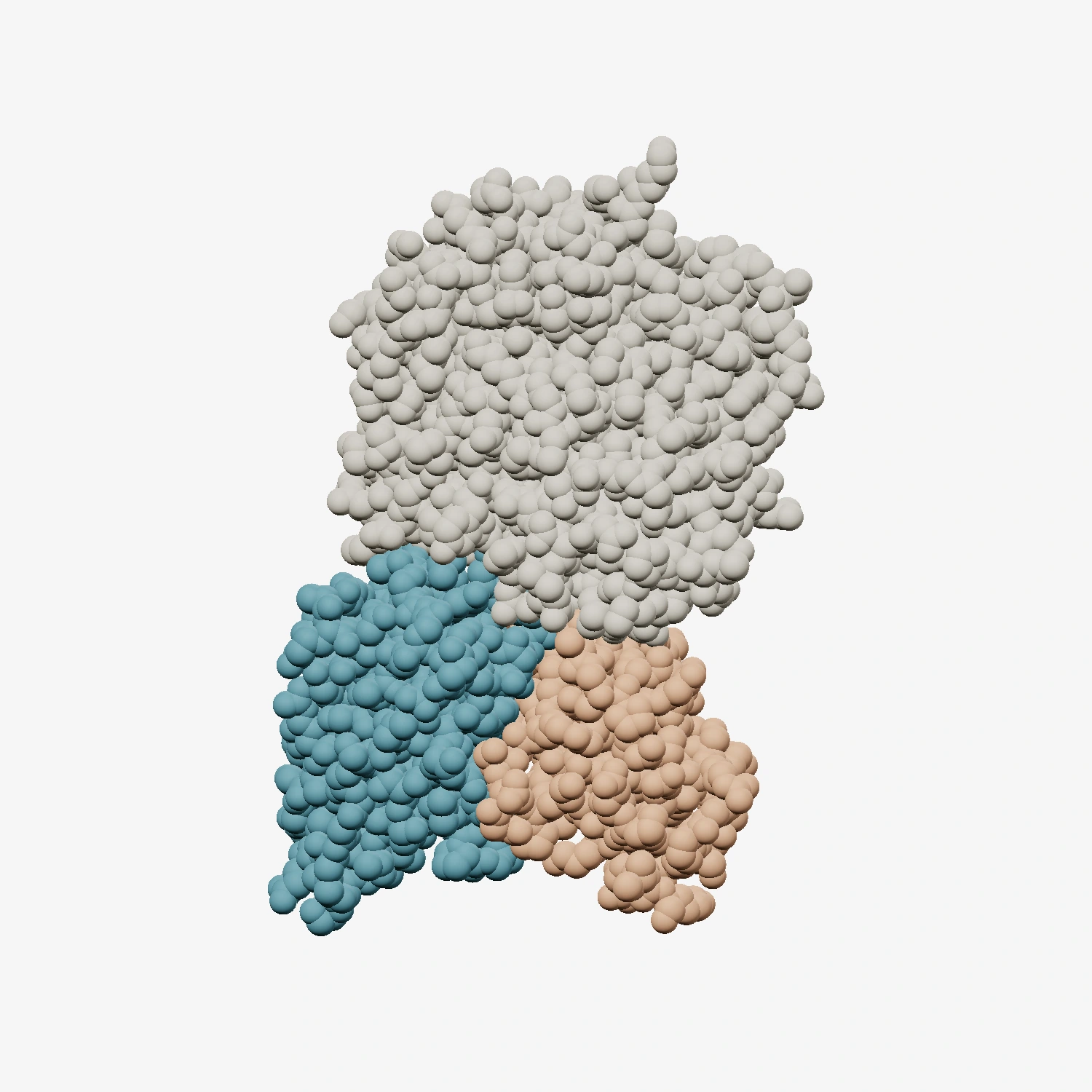
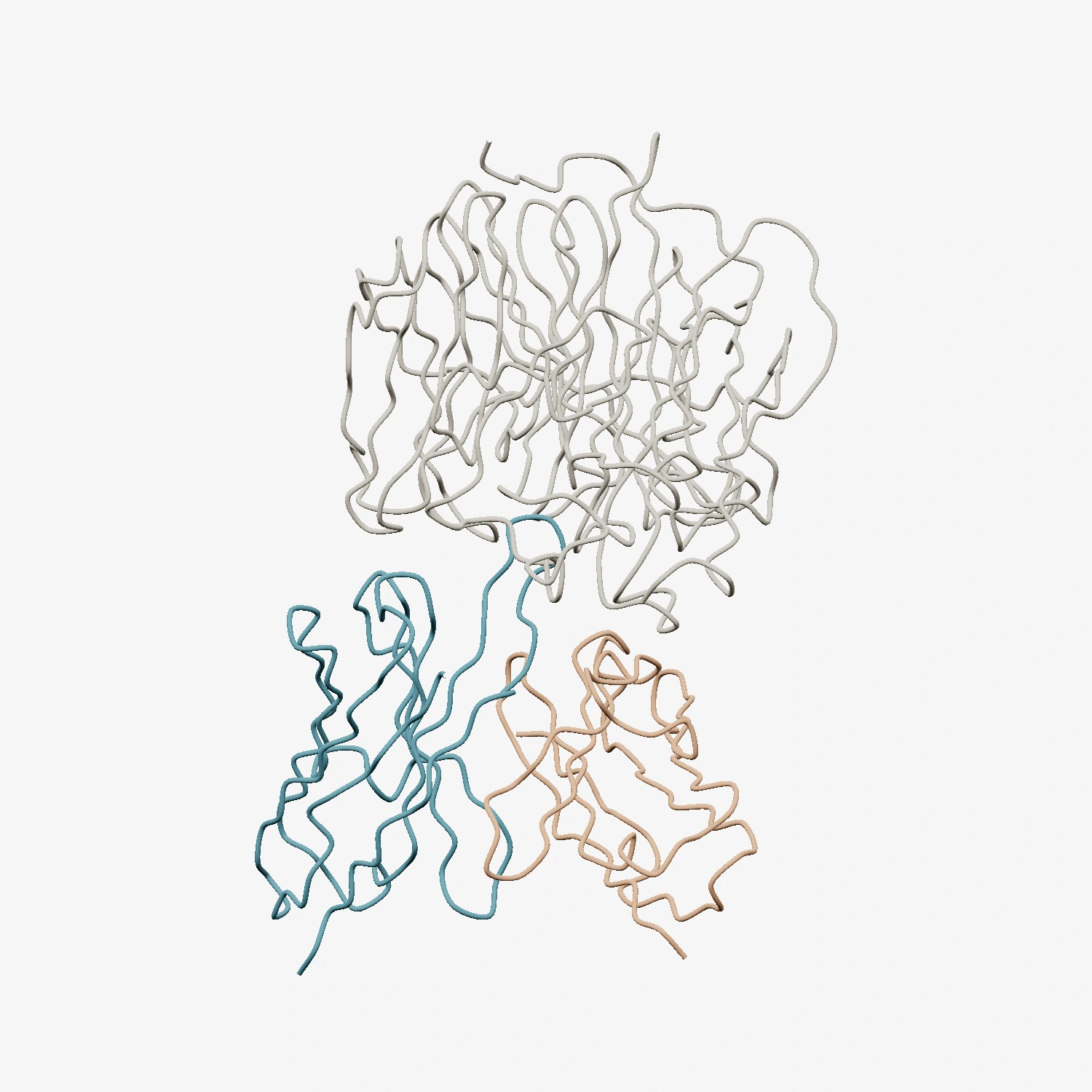
The native complex used as context for the paper’s Figure 3 (8yvn E I D). Space-filling atoms show the antibody–antigen interface; smoothed Cα traces reveal the three chains. Both views use the deposited cryo-EM atomic model and are fitted separately.
PDB 8YVN · cryo-EM atomic model ↗RCC represents a backbone segment by its Cα positions. A link is the displacement between neighboring positions: . With links, prescribed length , and fixed endpoint displacement , the allowed configurations form a bridge space:
This equation separates hard geometry from the rest of the design problem. A model may still need to learn favorable conformations, and a design objective may still need to reward contacts or penalize clashes. RCC makes the endpoints and Cα spacing exact on its regular coordinate domains. It does not make those other properties automatic.
The construction assumes a reachable endpoint, . The paper develops equal-length links. Its central question is how to parameterize this space so that generation, density evaluation, and gradient-based search can all use it. [§2.2]
Turn one global constraint into compatible local choices
Imagine cutting a chain into a left half and a right half. Once their meeting point is chosen, each half becomes a smaller fixed-endpoint problem. The whole chain can therefore be constructed by repeatedly making compatible splits.
For a parent segment from zero to , let the two children contain and links. The left child can reach a meeting point only if it lies within distance of the start. The right child must also be able to reach the endpoint from that same point. Their reachable regions overlap in a lens.
The coordinate domain stays the same when the endpoint displacement changes: choose a direction and a fraction of the available radius. The decoder accounts for the changing shape of the lens. Applying this rule to both children eventually reaches two- and three-link chains with explicit solutions.
Building an antibody loop
CAV-F6 · PDB 8YVN- 01Fixed anchors
- 02First split
- 03Recursive splits
- 04Completed loop
RCC constructs a backbone for the IMGT-defined H3 loop between anchors E96 and E113 in the deposited CAV-F6 complex. Dashed spans represent subchains waiting to be resolved; the final 17 Cα links are 3.8 Å long. These independently generated geometry examples use a simple clash-and-bend screen. The paper’s trained sampler was not used, and the candidates have not been validated as antibody designs.
Structure and loop annotation ↗Explore the geometry of a single split
Choose a split. Keep the bridge closed.
INTERACTIVE · 3D GEOMETRYThe general RCC framework asks each subtree to expose a compact summary. For a backbone, that summary is its endpoint displacement. The parent displacement is the sum of the two child displacements. If every local compatibility condition and every leaf has invertible coordinates, these maps assemble into a global encoder and decoder .
On the chosen regular domains, decoding always satisfies the bridge constraint, and encoding and decoding undo one another. A balanced tree gives linear total work and logarithmic parallel depth for fixed spatial dimension. This is a statement about the recursive construction, not a claim that the entire protein-design pipeline has logarithmic runtime. [Theorem 2.2]
Where the coordinate guarantee applies
The maps are exact and invertible on compatible regular charts. They are not one smooth global chart covering every possible bridge. A lens-center split has no unique radial direction; collinear subchains and boundary cases can also be singular. Appendix A.2 gives an example where a noncollinear overall bridge still encounters a singular intermediate split. The numerical checks and density formulas retain these regularity conditions.
Connect the coordinates to existing generators
A useful constraint representation should work with an existing generator. RCC supplies a retraction: a map that takes a generated backbone into the required bridge space and leaves an already-valid backbone unchanged, whenever the relevant normalization and charts are well defined.
For generated links , the first step distributes endpoint mismatch across the chain and normalizes every link to length b. This produces an equal-link source bridge q with its own endpoint displacement . RCC encodes that bridge, then decodes the same recursive coordinates under the required endpoint e.
This operation does not require retraining the underlying generator or changing its sampling procedure. It also does not minimize Cartesian displacement from the original sample: preserving recursive coordinates is a different choice from finding the nearest feasible backbone. [§2.3]
There are two distinct uses of the same geometry. The retraction above can close a sample after generation. During guided design, RCC can instead decode every candidate before it is evaluated. The second use is what prevents the optimizer from exploiting invalid geometry.
A coordinate density is not yet a backbone density
Equal-sized neighborhoods in coordinate space need not occupy equal amounts of backbone space. A decoder can stretch one region more than another. A normalized probability density over backbones therefore needs a volume correction.
RCC computes this factor through the same tree. Each node combines its children’s volume factors with the local meeting-point Jacobian and the amount by which both children deform when that point moves. This avoids constructing the full backbone decoder Jacobian.
The recursive volume calculation
For a subtree I, each matrix term projects onto directions in which a link can rotate without changing its length. Their sum describes how those rotations can move the subtree endpoint. At a regular split, the two children contribute jointly:
The total work is O(Nd³), with O(d³ log N) parallel depth. For proteins, d = 3 is fixed. This factor is needed for normalized densities; a geometry-only guidance implementation can omit it when the loss does not use density. [Theorem 2.4]
The paper checks these identities independently. Across 240 prespecified protein-bridge configurations with 2–31 links, the maximum float64 constraint residual is 4.07 × 10⁻¹⁵. Recursive log volume agrees with the full decoder Jacobian to 1.42 × 10⁻¹⁴, and coordinate gradients to 1.91 × 10⁻¹⁴. These checks establish numerical agreement on tested regular domains, rather than empirical protein quality. [Table 6]
Score the backbone that can actually be built
A learned sampler maps base noise ε into coordinates u using . The backbone decoder turns those coordinates into a valid chain. Guidance changes the base noise to improve a differentiable design objective:
- Initialize. Draw four candidates from the learned conditional proposal.
- Decode and score. Construct a valid backbone for each candidate before evaluating its contacts, sterics, and local geometry.
- Update. Take 15 Adam steps through the sampler and decoder, retaining the best objective encountered.
Scoring the initial candidates and every update gives 4 × (15 + 1) = 64 feasible objective evaluations per condition. The prospective study withholds the native H3 sequence and coordinates from the model, design objective, ranking, and success criteria. Native RMSD is reserved for retrospective analysis. [Algorithm 2]
What the experiments show
The first evaluation asks how much closing existing generator outputs changes their structural summaries. RCC is applied to 20,610 LoopGen CDR samples, 212,940 CATH fragment samples, and 292 FrameFlow motif-linker samples. All 233,842 outputs satisfy the reported geometric feasibility criterion.
Compared with fixed-512 projection on the same inputs, changes in each setting’s primary structural measure are below 0.01 Å. That is a comparison between closure procedures, not a claim that each backbone moves by less than 0.01 Å from its raw generated state. On CATH, RCC uses one fixed encode–decode pass; FABRIK has the lowest reported p99 latency. [Tables 1–2]
Prospective antibody-loop design
The main guidance study uses a PDB-disjoint temporal panel of antibody–antigen complexes. The checkpoint and evaluation protocol were fixed before the temporal test structures were accessed. Of 292 initial conditions, four fail the prespecified eligibility criteria, leaving 288 conditions from 255 PDBs, with H3 lengths of 6–26 residues.
- Design conditions
- 288
- Parent PDBs
- 255
- Evaluations / condition
- 64
The learned proposal assigns native loops higher density than uniform coordinates in 92.0% of conditions. Permuting context across PDBs lowers mean native-loop log density by 1.152 nats, with the matched context preferred in 61.3% of conditions. The model is using information about the surrounding antibody and epitope, beyond a length-and-endpoint description alone.
Learning helps. Feasible guidance adds more.
PROSPECTIVE · TABLE 3
See the structural metrics
| Policy | Objective ↓ | Cα clean ↑ | Diversity (Å) ↑ | Native RMSD (Å) ↓ |
|---|---|---|---|---|
| Uniform sampling | 0.59156 | 28.13% | 11.102 | 9.063 |
| Learned sampling | 0.10703 | 81.60% | 5.343 | 5.564 |
| RCC guidance | 0.01653 | 98.61% | 5.841 | 6.008 |
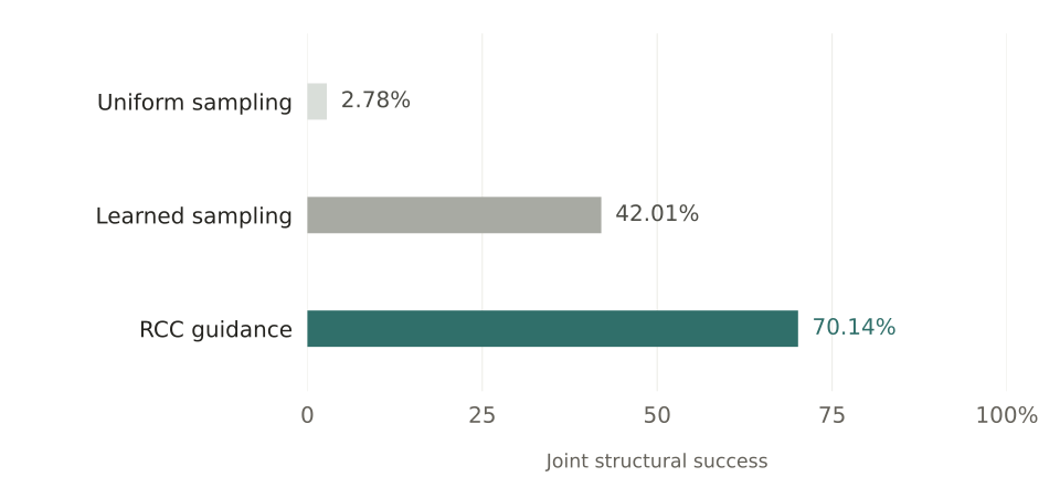
Learning the proposal raises structural success from 2.78% to 42.01%; coordinate guidance raises it to 70.14%, an increase of about 28 percentage points over learned sampling. Every one of the 18,432 backbones evaluated during guidance satisfies the endpoint and link-length constraints. The objective improves over learned sampling on 278 of 288 conditions. [Appendix E.1]
The result is not native-loop reconstruction. Mean native Cα RMSD rises from 5.564 to 6.008 Å under guidance, while diversity rises from 5.343 to 5.841 Å. The objective favors the paper’s context-directed structural criteria rather than similarity to the withheld native H3.
Why optimizing first and repairing later falls short
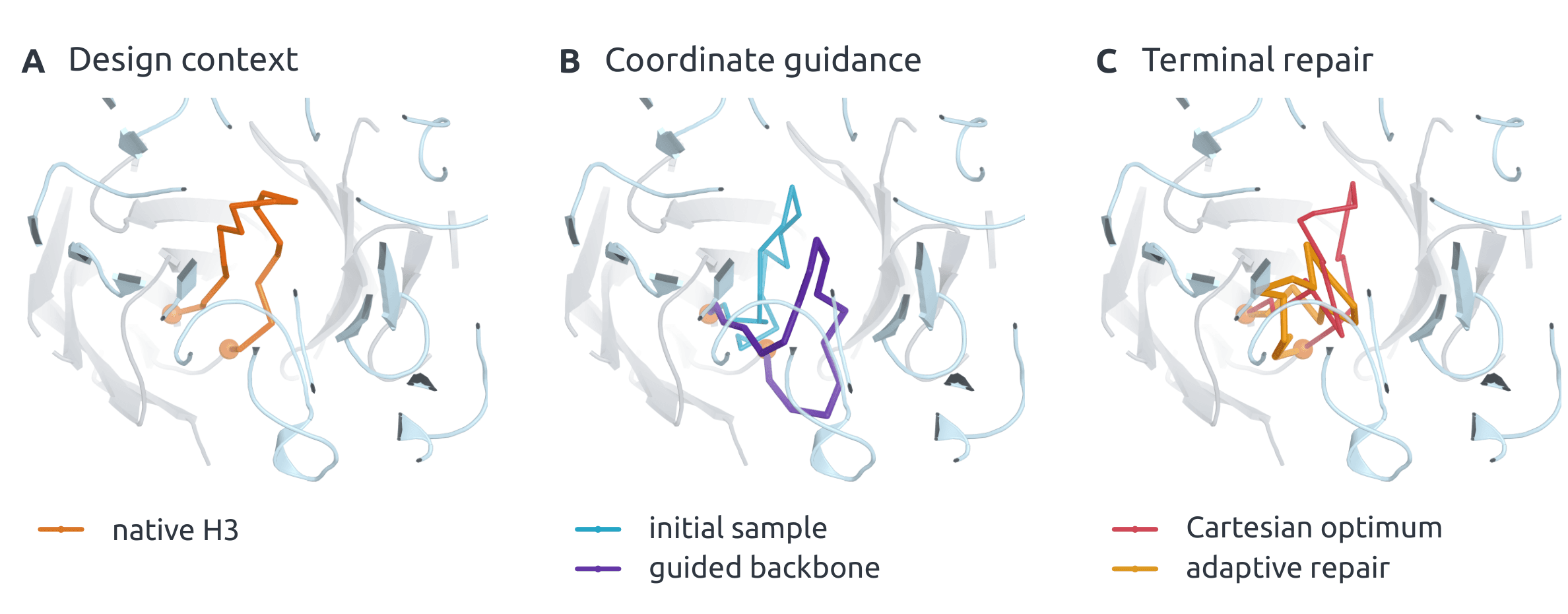
A useful control keeps the starting candidates and scoring budget fixed, then changes the space in which optimization runs. The paper repeats the same four-start, 15-step search in Cartesian link coordinates and repairs the final candidates afterward.
Before repair, the Cartesian search reaches a lower mean objective than RCC guidance: 0.00755 versus 0.01653. But those candidates violate the bridge constraints, with a maximum normalized link error of 3.41. Their apparently better score belongs to geometry that the final design is not allowed to have.
Repair restores geometry, but loses the score.
POST HOC · TABLE 20
Compare success after each repair method
| Search and terminal map | Structural success ↑ | Cα clean ↑ |
|---|---|---|
| RCC-coordinate guidance | 70.14% | 98.61% |
| Cartesian + adaptive projection | 7.64% | 48.61% |
| Cartesian + FABRIK | 6.60% | 45.49% |
| Cartesian + CoBarS | 6.94% | 44.79% |
| Cartesian + RCC retraction | 11.11% | 53.47% |
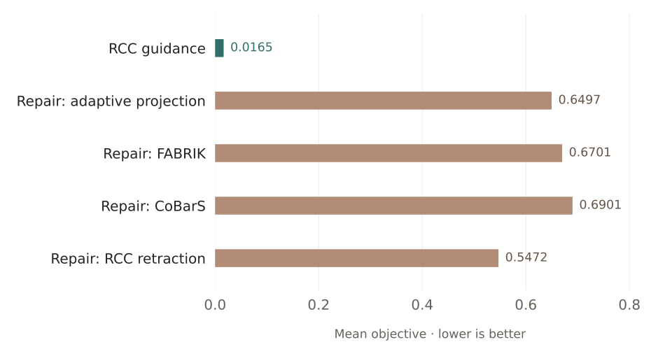
All four terminal methods restore valid geometry. None preserves the objective improvement: structural success after repair ranges from 6.60% to 11.11%, compared with 70.14% for direct coordinate guidance. Even the RCC retraction performs poorly when used only at the end. The distinction is maintaining feasibility during search, not simply choosing RCC as the final correction.
This control is post hoc. It matches initial samples and objective-evaluation count, not total computation. It also does not establish superiority over every method that keeps candidates feasible throughout optimization. That comparison is a separate question.
Exact geometry leaves important design questions open
The stronger feasibility-maintaining controls make the conclusion more precise. In a separate development comparison, RCC-coordinate guidance performs comparably to Riemannian guidance and Adam differentiated through closure. Across three proposal-training seeds, the RCC-minus-Riemannian difference in the combined structural-and-steric criterion is −0.95 percentage points, with a descriptive 95% interval of −7.31 to +5.39 points. The paper does not establish a general optimization advantage over these methods. [Appendix E.5]
Backbone resolution also matters. The original guidance objective improves Cα cleanliness, yet the reconstructed atom-level clean fraction is lower than for learned sampling. A later atom-aware objective changes that tradeoff:
Cα cleanliness is not atom-level cleanliness.
POST-HOC CHECK · TABLE 23| Policy | Cα clean ↑ | Reconstructed atom clean ↑ |
|---|---|---|
| Learned samplingProspective outputs | 81.60% | 23.26% |
| RCC guidanceProspective outputs | 98.61% | 19.79% |
| Atom-aware RCC guidancePost hoc | 100.00% | 75.00% |
Independent sequence-design and refolding checks are more demanding still. In the first development pilot, none of the 64 sequence attempts for RCC-coordinate Adam comes within 2 Å of its designed H3 backbone after refolding. The other guided methods also have zero passing attempts. Exact closure and good coarse structural scores do not establish sequence–structure self-consistency. [Table 26]
A later, distinct endpoint-conditioned generation experiment reports 24 of 128 sequence attempts passing the same 2 Å criterion with synchronized atoms, across 11 of 32 PDBs. These are development results from a different pipeline, not an update to the prospective 70.14% figure. The native-sequence controls perform substantially better, training-set overlap with the refolding model is unresolved, and none of these experiments measures physical folding or binding. [Table 28]
A reusable construction for constrained design
The recursive idea is broader than chain geometry. The paper also considers allocating a fixed budget among bounded variables. Each subtree only needs to expose its subtotal. At a split, the permitted left subtotal is the interval that satisfies the left bounds while leaving a feasible amount for the right:
The allocation study validates coordinates and volume factors on 312 instances with 2–40 variables. On 8,192 unseen outputs of a frozen predictor, the maximum total-budget error falls from 0.1915 to 7.11 × 10⁻¹⁵, without a component-bound violation. Euclidean projection has slightly lower prediction RMSE on those same outputs. Exact constraints and prediction accuracy remain distinct objectives. [Tables 29–30]
For programmable biology, RCC offers a way to separate learned design preferences from geometric requirements that every candidate must satisfy. A generator supplies proposals; a coordinate system enforces the specified constraints; an objective guides the search within them. Better biological objectives and experimental evidence are still needed to turn those valid structures into useful designs.