
Learning transferable free energies
Fisher-conditioned flow matching for generalization across molecular transformations
Deciding which molecule to make next often means comparing candidates that differ by only a few atoms. Those changes can alter how a molecule interacts with its surroundings. Free-energy calculations help quantify such differences, but each comparison requires sampling many molecular configurations.
A model that learns from many such calculations could make that work reusable. There is a subtle obstacle: the coordinate normally used to describe a transformation tells us how the energy function changes, not how much the molecular distribution has changed. A point labeled “halfway” need not represent comparable progress in two different transformations.
This work tests a coordinate based on the change in those distributions. Fisher information provides a way to measure that change, giving a shared flow model a more consistent description of progress along each path. The study asks whether this helps on molecular pairs absent from training; it still uses simulation data from those held-out pairs to construct the coordinate.
 View full-size figure
A shared coordinate for different transformations. The same coupling value can correspond to different amounts of distributional change. Normalized Fisher arc length instead measures fractional progress along each pair’s information-geometric path. The paths and profiles in this original figure are schematic, not molecular trajectories or measured Fisher profiles.
Figure 1 in the Fisher flow matching paperThe same input can mean different things
In an alchemical calculation, one molecular system is gradually transformed into another through a sequence of intermediate energy functions. These intermediates provide a computational path between the endpoint distributions.
The coupling parameter λ labels that sequence: λ = 0 is one endpoint and λ = 1 is the other. Molecular dynamics samples the intermediate distributions, and thermodynamic integration combines their average energy derivatives into a free-energy difference.
The learning problem is to train one model across many transformations and apply it to a pair absent from training. That requires the model to understand both which pair it is working on and where it is along that pair’s path.
Raw λ gives every pair the same numerical interval, but it does not make their intermediate distributions comparable. A small step in λ may barely change one system and substantially change another. The paper asks whether a coordinate based on distributional change can make that shared learning problem easier. [1, §2]
Measure how much the distribution changes
Fisher information measures how sensitive a probability distribution is to a change in its parameter. Along an alchemical path, it is proportional to the variance of the same energy derivative used in thermodynamic integration. We write it as 𝓘 to distinguish it from free energy.
Where a distribution changes rapidly, Fisher length accumulates quickly. Where it changes slowly, the same λ increment contributes less length. The result is unchanged by a smooth monotonic relabeling of the path.
Locally, the Kullback–Leibler divergence between neighboring distributions is approximately ½𝓘(λ)(dλ)² = ½(dℓ)². Equal small steps in unnormalized Fisher length therefore correspond to equal leading-order local divergence. This is a local relationship; cumulative path length is not generally the finite KL divergence between the endpoints.
The implementation uses normalized length, ℓ̄ = ℓ/ℓmax, so every pair’s coordinate runs from zero to one. That choice matters because total lengths vary from 0.41 to 11.79 in the small-molecule corpus. Normalization aligns fractional progress along each path; it does not make the absolute information distance equal across pairs with different total lengths. [1, §3.2–3.3]
Compare the same input across two paths
Change near the end
λ 0.50Fisher progress 38%
Change near the start
λ 0.50Fisher progress 63%
The coordinate is only as good as its energy derivative
Alchemical simulations often soften interactions near the endpoints to avoid singular energies when atoms appear or disappear. Under a linear interpolation of endpoint energies, ∂λU equals UB − UA. A softcore Hamiltonian generally does not obey that identity.
Evaluating the endpoint difference on configurations sampled under softened interactions can produce extreme outliers: overlaps that are harmless in the sampled system become severe clashes in the fully interacting endpoint. Such errors contaminate both the thermodynamic-integration target and the variance used to construct Fisher length.
The paper instead evaluates a centered finite difference of the actual softcore Hamiltonian, with δ = 0.01 and one-sided differences at λ = 0 and 1. Both conditioning modes use that same corrected derivative. This isolates the coordinate comparison from errors introduced by an inconsistent energy estimator. [1, §3.5]
Evaluate transfer on held-out molecular pairs
The main chemistry experiments use five-fold cross-validation. Each fold withholds complete molecular pairs, and each configuration is trained with three seeds and evaluated with three sampling seeds. The raw-λ and Fisher-conditioned models share architecture, training data, optimizer settings, batches, and seeds.
The target is each held-out pair’s own simulation-derived ΔF. Absolute prediction errors are measured in kJ/mol. The aggregate percentage reduction compares the sum of errors under the two coordinates; a positive value favors Fisher conditioning. A pair counts as a win only when its error is less than 95% of the other mode’s error. Ties are excluded from the reported decided win rate.
A Lennard–Jones diagnostic provides a controlled physical example. Four training pairs use particle-size ratios σB/σA from 1.05 to 1.20; the held-out pair uses 1.30. The reported error falls from 1.70 ± 0.59 to 0.35 ± 0.19 kJ/mol, a reported 79.5% reduction. This is an extrapolation test on a simple interaction model, not a drug-binding benchmark. [1, §5.1]
A measurable gain—and a useful feature tradeoff
The small-molecule corpus contains 129 transformations across alkanes, alkylaromatics, alcohols, amines, thiols, and a heterogeneous remaining group. These are single-topology substituent extensions simulated in vacuum at 300 K, with AM1-BCC charges and the OpenFF Sage force field.
With a transformer and atom-count features, Fisher conditioning reduces aggregate held-out error by 5.6%, with a reported 95% interval of 0.8% to 9.9%. It wins 73 of 114 decided comparisons; the other 15 pairs are ties. The architecture and feature ablations show that this benefit is not universal.
| Architecture / features | Fisher wins / decided | Error reduction | Reported 95% CI |
|---|---|---|---|
| MLP Atom counts | 51 / 94 | +0.6% | [−1.9, +3.3]% |
| MLP Morgan fingerprints | 59 / 107 | +0.3% | [−4.7, +4.9]% |
| Transformer Atom counts | 73 / 114 | +5.6% | [+0.8, +9.9]% |
| Transformer Morgan fingerprints | 60 / 116 | −2.0% | [−11.7, +6.7]% |
Morgan fingerprints improve the transformer’s absolute errors under both coordinates. Yet their inclusion removes the additional advantage of Fisher conditioning. The authors interpret this as partial substitution: chemical similarity features may already supply information that the geometric coordinate would otherwise contribute.
| Pair features | Raw λ | Fisher coordinate |
|---|---|---|
| Atom counts | 7.66 | 7.24 |
| Morgan fingerprints | 4.83 | 4.93 |
The distinction is useful when interpreting the result. The transformer with atom counts is the clearest test of the coordinate hypothesis in these experiments. It is not the configuration with the lowest absolute errors among all reported feature choices.
The advantage depends on a meaningful molecular mapping
The second chemistry study uses transformations drawn from six target subsets of the pmx protein–ligand benchmark. Of 165 selected edges, 32 fail during system construction or simulation, leaving 133 usable pairs. The failures include 20 molecular-dynamics crashes and 12 charge-assignment failures.
This experiment uses newly run vacuum simulations. Its evaluation targets are those simulations’ ΔF values, not the published pmx binding free energies. It therefore tests generalization across drug-like transformations without establishing binding-affinity accuracy against experiment.
The main comparison focuses on 79 pairs with fewer than 30% of atoms in the alchemical region. These mappings retain a substantial shared molecular core. On that subset, the transformer with atom counts yields an 11.5% aggregate error reduction, with a reported 95% interval of 3.3% to 19.0%, and wins 46 of 69 decided comparisons.
| Architecture / features | Fisher wins / decided | Error reduction | Reported 95% CI |
|---|---|---|---|
| MLP Atom counts | 27 / 56 | −1.3% | [−4.4, +2.0]% |
| MLP Morgan fingerprints | 32 / 63 | −1.4% | [−5.2, +1.8]% |
| Transformer Atom counts | 46 / 69 | +11.5% | [+3.3, +19.0]% |
| Transformer Morgan fingerprints | 9 / 41 | −6.5% | [−10.0, −3.6]% |
When the maximum-common-substructure mapping fails to retain a meaningful shared core, the pattern changes. Among 35 pairs with at least 70% alchemical atoms, the same configuration has a 50% decided win rate and a −3.1% aggregate reduction: Fisher conditioning is slightly worse in aggregate. The coordinate helps within the reported operating regime; it does not repair a poor molecular mapping.
Where Fisher conditioning helps
pmx · Transformer + atom counts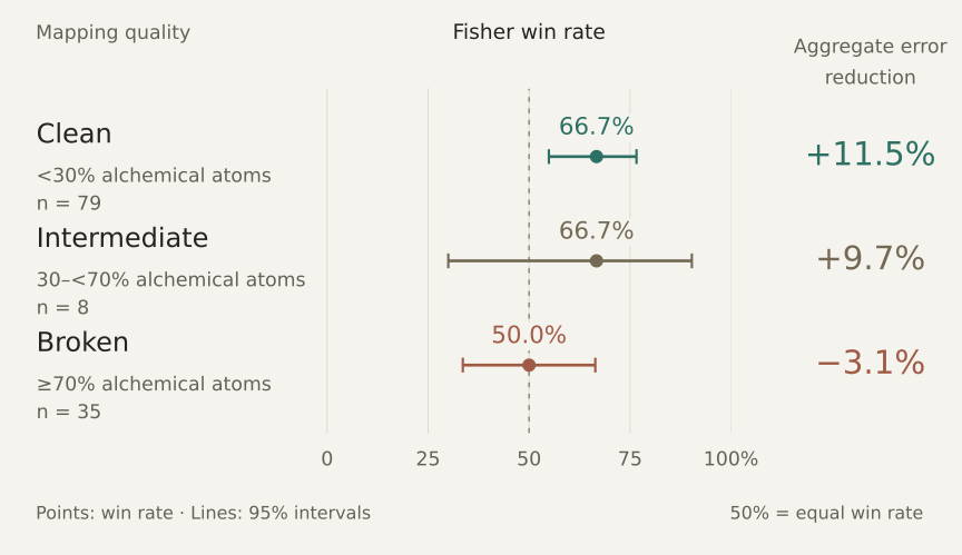
Values and source
| Mapping group | Group size (n) | Decided win rate | 95% interval | Aggregate error reduction |
|---|---|---|---|---|
| Clean <30% alchemical atoms | 79 | 66.7% | 54.9–76.6% | +11.5% |
| Intermediate 30–<70% alchemical atoms | 8 | 66.7% | 30.0–90.3% | +9.7% |
| Broken ≥70% alchemical atoms | 35 | 50.0% | 33.6–66.4% | −3.1% |
Win rates and interval endpoints were recovered from the original vector figure and rounded to 0.1 percentage point. The intervals were not recalculated. Group sizes include ties and are not the denominators for decided win rates. Aggregate error reduction compares sums of absolute errors.
Download values and provenance ↗The paper also tests whether the square root in Fisher length matters. Replacing ∫√𝓘 dλ with ∫𝓘 dλ gives a −2.4% reduction, with a reported interval of −9.6% to 4.0%, compared with +6.5% for the canonical coordinate on the same 111-pair comparison. This supports the specific geometric construction rather than an arbitrary rescaling of λ. [1, §6]
Toward broader transfer in molecular modeling
The contribution is a concrete way to connect physical geometry to the inputs of a generative model. A coordinate that reflects distributional change can remove some of the mismatch that a shared model would otherwise need to learn from molecular descriptors alone.
Several steps remain before that becomes a replacement for a full free-energy workflow. The model would need a Fisher profile estimated from molecular features or a limited pilot simulation, rather than the held-out pair’s full simulation data. Broader validation would also require explicit solvent, appropriate hybrid topologies, improved atom mapping, and the protein-bound portion of the alchemical cycle.
For programmable biology, this work addresses one part of molecular design: learning physical quantities across related chemical systems. Its results motivate more transferable estimators while keeping the scope precise—scalar energy-derivative modeling under a stated simulation protocol, with benefits that depend on the architecture, features, and quality of the molecular path.